
The following is a guest post from Spring Valley Asset Management:
Disclaimer: While investment in managed futures can help enhance returns and reduce risk, it can also do the opposite and result in further losses in a portfolio. In addition, studies conducted on managed futures as a whole may not be indicative of the performance of any individual CTA. The results of studies conducted in the past may not be indicative of current periods.
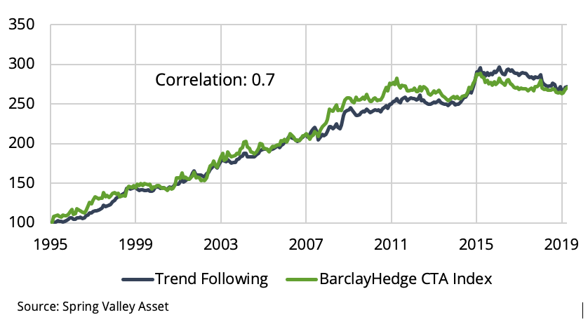
Commodity Trading Advisors (CTAs) are a class of hedge funds that trade primarily in liquid global futures markets. These include currencies, fixed income, equity indices, and commodities. CTAs pursue many different types of strategies. However, research has shown that they predominantly follow trends. Trend following buys assets that have risen in price and sells assets that have fallen in price. The strategy has been robust historically and consistent across asset classes. Using the approach in [1], we construct a proxy trend following strategy. In Exhibit 1, we confirm that our proxy strongly correlates with the BarclayHedge CTA Index.
Exhibit 1
CTAs are mostly trend followers
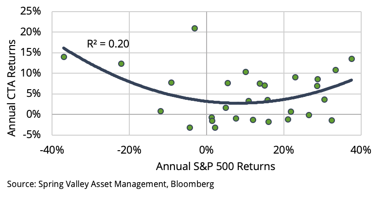
CTAs have provided valuable diversification to both traditional and alternative asset classes. They are best known for their performance during “crisis” periods. A crisis occurs during significant, sustained declines in equity markets. As shown in Exhibit 2, CTA’s have performed well during large moves, higher or lower, in the equity markets. This convex relationship has come to be known as the “CTA smile.”
Despite their diversification benefits, CTAs have struggled over the past ten years. Low volatility, high correlations, and suppressed interest rates are the most common explanations. We will explore the validity of these claims.
Exhibit 2
CTA Smile
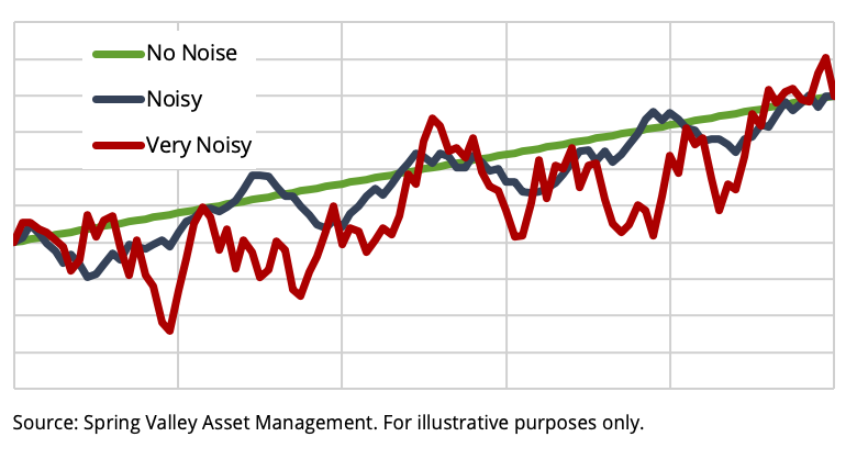
Since CTAs generally follow trends, we can hypothesize that trends have weakened over the last ten years. As shown in Exhibit 3, trends come in many different forms. Some trends are easy to identify and exhibit little noise, while others are very noisy, making it difficult to detect the underlying trend.
Exhibit 3
Trends come in many different forms
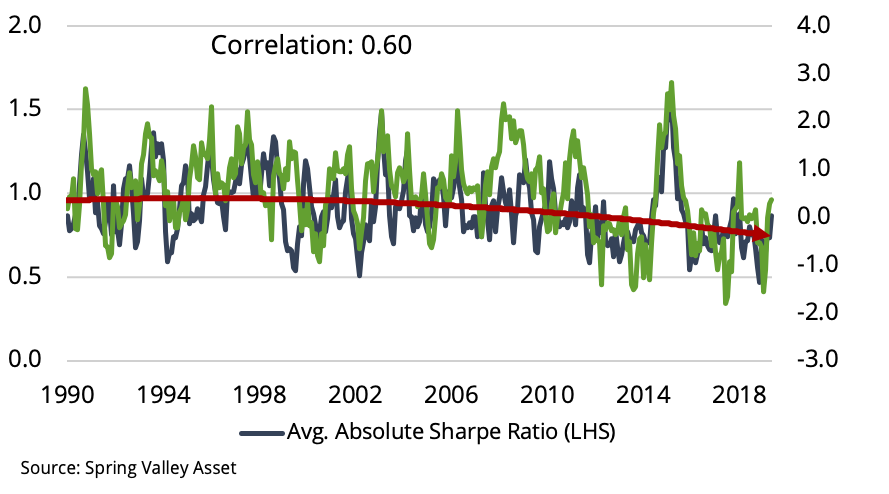
To quantify the strength of a trend, we calculate the rolling 12-month absolute Sharpe ratio of each underlying market. We then take the average values across 60 markets from four asset classes. Exhibit 4 plots the rolling 12-month Sharpe ratio of the BarclayHedge CTA index against our aggregated measure of trend strength. As expected, the two series are highly correlated. CTAs perform well when there are strong trends. However, it is also evident that the trend’s strength has steadily declined. Since the Sharpe ratio consists of return and volatility, we will determine the role of each component in weakening trends.
Exhibit 4
CTAs perform well when there are strong trends
Since trend following has a convex relationship to stocks and bonds, the general interpretation is that it is long volatility. For example, the features of trend following have been replicated using an options strategy that buys put and call options [2]. However, we can reason that strong trends can form independent of volatility. For example, consider an asset that rises 1% every day. Despite having no volatility, it is a powerful trend. Also, consider an asset that alternates daily, increasing 10% and falling -10%. Despite displaying very high volatility, trend following would perform quite poorly.
Exhibit 5
CTA performance across volatility regimes
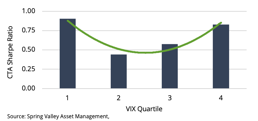
We can empirically determine the relationship between volatility and CTA performance. As in [3], we will use the VIX index. The VIX measures the market’s expectation of near-term volatility implied by S&P 500 index options. This makes our analysis comparable to the CTA smile. Also, the most common explanations for low volatility, such as monetary policy and sluggish growth, are priced in the VIX.
We take the average VIX level each quarter and then split the observations into quartiles. Exhibit 5 shows the realized Sharpe ratio of CTAs within each quartile. We notice that CTAs perform very well in the highest VIX quartile. This is intuitive since CTAs perform well during significant equity market declines. However, inconsistent with the logic that trend following is long volatility, CTAs also perform well in the lowest VIX quartile. It also supports our sense that trends can develop independently of volatility levels.
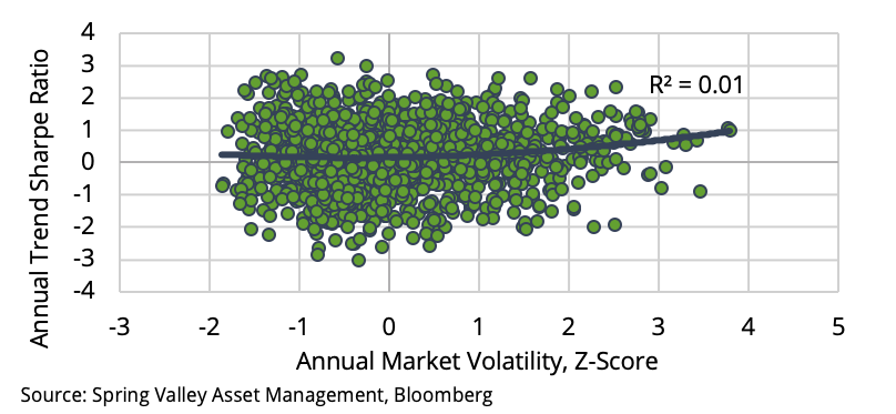
Also, we can observe the relationship directly. We calculate the annual volatility of each market and standardize them over time using z-scores. We then calculate the annual Sharpe ratio of trend following performance in each market. As shown in Exhibit 6, the link between performance and volatility is relatively weak. If anything, the shape of the trendline is convex, resembling the relationship between the VIX and CTA performance. Our analysis is consistent with the work of [3, 4], who also found the relationship between volatility and trend following to be tenuous. Therefore, our results suggest that the lack of volatility over the recent decade is a weak explanation for the underperformance of CTAs.
Exhibit 6
Strong trends can form independent of volatility
We have shown that trends can develop in both low and high-volatility environments. The absolute size of the returns has declined in the recent decade. This result would be consistent with [5].
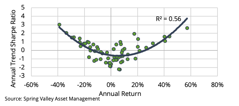
Research shows that significant cumulative returns in the underlying market produce a strong performance for trend-following strategies [6]. As a demonstration, we simulate our trend-following strategy on a random walk. The random walk is unpredictable, and a trend-following strategy is expected to yield a Sharpe ratio of zero. However, in Exhibit 7, we observe a robust convex relationship. Trend following performs well during significant cumulative moves in the underlying.
Exhibit 7
Trend following applied to a random walk
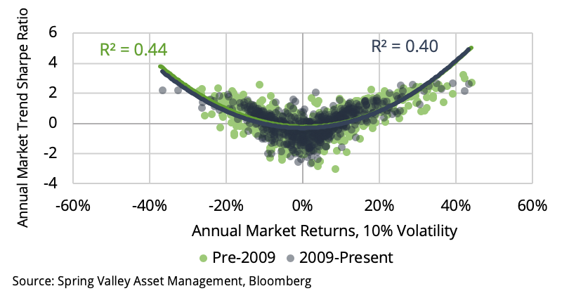
To quantify this effect over our sample, we normalize the daily returns of each market in our universe to 10% volatility. In Exhibit 8, we display the relationship between the annual trend following performance applied to each market and the annual returns of the underlying market. We show the results for the periods before and after 2009. We observe that the relationship has remained stable. Therefore, the underlying dynamics that drive trend following profitability still exist. Also, as in [5], we can conclude that there is no indication of a change in the strategy’s ability to capture trends.
Exhibit 8
Trend following still “works,” but it requires large cumulative moves
However, Exhibit 9 shows the distribution of annual returns across all markets for both periods. The past decade has seen a much narrower distribution. In other words, there have been much smaller trends and, therefore, the ability of CTAs to deliver outsized performance. While volatility has declined, the absolute size of returns has contracted even more.
We have shown that CTAs have a very strong relationship with the strength of trends across individual markets. While volatility has been cited as a reason for poor CTA performance, we find that it has little relationship to the performance of trend following.
A strong trend can form in both high and low-volatility environments. We then investigated the absolute size of returns in the underlying markets, which have a much stronger relationship to trend following performance. While CTAs have still been able to capture trends, the trends have been much smaller. This has been the determining factor for CTA performance in the recent decade.
In addition to low volatility, correlations have been used to describe recent CTA underperformance. For directional trading strategies like trend following, if the performance across markets is perfectly correlated, the strategy would not realize any diversification from trading multiple markets. If performance is uncorrelated, the strategy’s performance should scale with the square root of the number of markets.
Exhibit 9
The number of large moves has decreased in the last decade
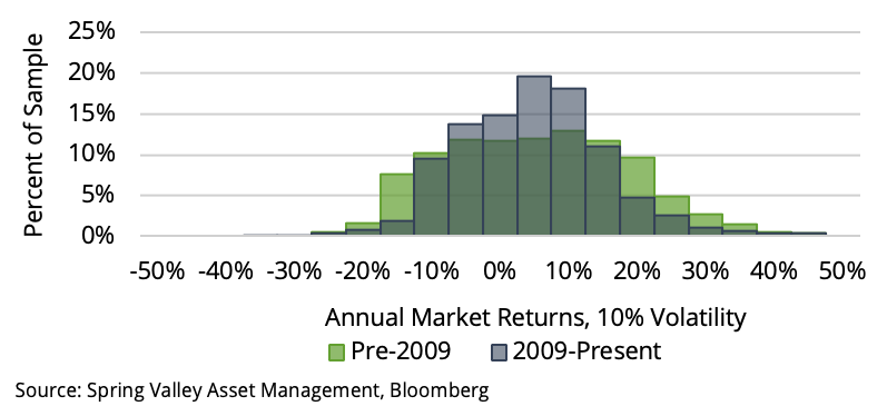
Exhibit 10
Correlations have been relatively higher over the recent decade
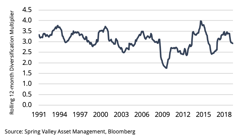
Exhibit 11
Diversification multipliers are not substantially different across samples
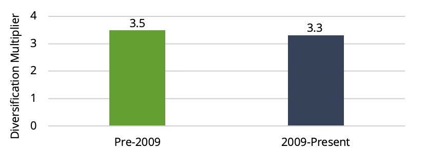
Using our trend-following proxy, we can calculate the impact of higher correlations in the recent decade. We can estimate the Sharpe ratio of our trend-following portfolio by scaling the average Sharpe ratio across all individual market trend strategies by a factor called the diversification multiplier. A higher multiplier indicates a more diversified portfolio. In Exhibit 10, we show the rolling 12-month diversification multiplier. We can see that it has been lower over the past decade. In Exhibit 11, we calculate the diversification multipliers before and after 2009. While the most recent decade has seen lower diversification, the impact on performance is marginal. It translates to only a 6% decrease in the Sharpe ratio. This is consistent with the results in [5]. We can say that high correlations have not been responsible for the decline in CTA performance over the whole period.
We also examine the relationship between correlation environments and CTA performance. Each quarter, we calculate the average absolute correlation across markets and the realized Sharpe ratios for CTAs in each quartile. In Exhibit 12, we observe that the relationship resembles that of volatility. Conceptually, volatility and correlation are linked. An increase in volatility across markets indicates an increase in systematic risk. Correlations also increase if systematic risk increases and asset-specific risk remains the same.
These observations are consistent with the work in [7], which studies the performance of CTAs across volatility-correlation regimes. We split our observations for volatility and correlations into two buckets: those above and below the sample median. In Exhibit 13, we show the performance of each overlapping state. When volatility and correlation are both high or low, CTAs have delivered strong performance.
Exhibit 12
CTA Performance across Correlation Regimes
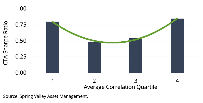
Exhibit 13
CTA performance across volatility and correlation regimes
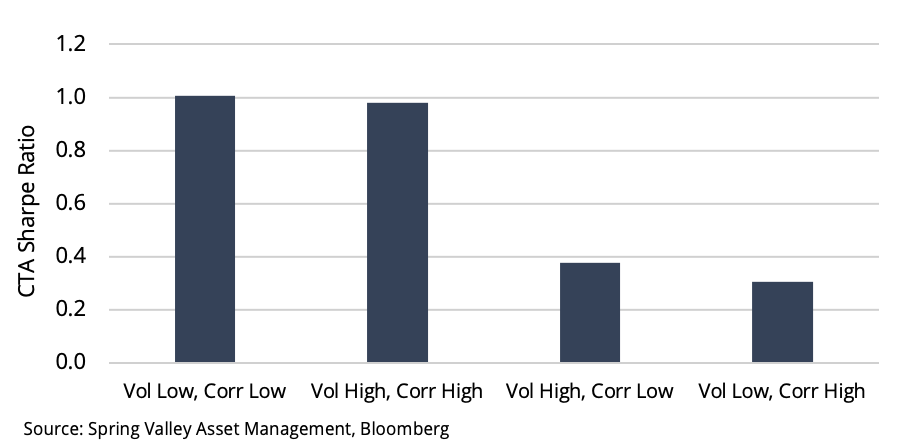
We can conceptualize why CTAs perform well when correlation and volatility are high and low. An environment where both are high generally coincides with a crisis. An extended period of deleveraging increases the persistence of trends. Since they are highly correlated, the effect is pervasive. On the other hand, the ideal environment for CTAs is when both are low. In low-volatility environments, prices are slow to absorb new information, which results in trends. This information also diffuses slowly across related markets. CTAs can also achieve greater diversification from lowly correlated markets.
Finally, we explore the impact of low cash rates. Futures trading involves posting a margin against a portion of the underlying value of the contract. The collateral return is the return accruing to the margin held against a futures position, generally the U.S. T-bill rate. Also, excess cash can be invested elsewhere, traditionally in short-term Treasuries. When interest rates are high, interest income from these sources can be substantial.
Exhibit 14
Returns on cash have been much lower
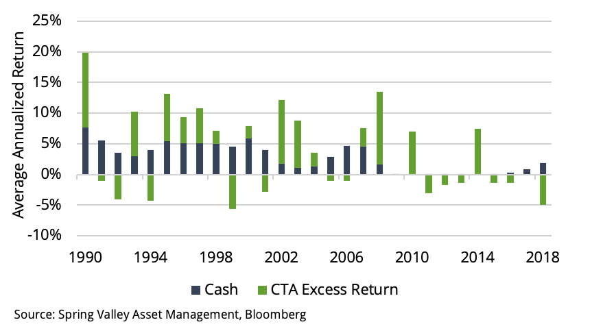
Exhibit 14 plots the annual return on 3-month T-Bills for each year and the annual excess returns of CTAs. Over the past decade, rates have been about zero, whereas in years prior, CTAs had a significant tailwind from interest earned on cash.
The CTA industry has performed poorly over the last ten years. We have found the culprit to be the weakening of trends, which is the result of smaller absolute moves across markets. However, a simple trend-following strategy has still been able to capture the strong trends that have occurred. If these significant moves return, and we believe they will, trend following should capitalize on them. In addition, we believe CTAs continue to provide important diversification benefits as part of a broader institutional portfolio.
References
- Palatiello, 2019, The average is better than average
- Fung, D. A. Hsieh, 2001, The Risk in Hedge Fund Strategies: Theory and Evidence from Trend Followers, The Review of Financial Studies 14(2), 313-341.
- Fan, I. Kleshchelski, 2017, Trend Following and Volatility Regimes (PDF)
- Malek, S. Dobrovolsky, 2006, Volatility Exposure of CTA Programs and Other Hedge Fund Strategies
- Babu et al., 2019, You Can’t Always Trend When You Want
- Capital Fund Management, 2018, The Convexity of Trend Following,
- Sabar, 2013, When Do Trend Followers Make Money?
Disclaimer
The information has been obtained or derived from sources believed by the authors and Spring Valley Asset Management, LLC (“SVAM”) to be reliable. However, the authors and SVAM do not make any representation or warranty, express or implied, as to the information’s accuracy or completeness, nor does SVAM recommend that the attached information serves as the basis of any investment decision. This document has been provided to you for information purposes. It does not constitute an offer or solicitation of an offer, or any advice or recommendation, to purchase any securities or other financial instruments and may not be construed as such. This document is intended exclusively for the use of the person to whom it has been delivered by SVAM and is not to be reproduced or redistributed to any other person. This document has been prepared solely for information purposes. The information contained herein is only current as of the date indicated and may be superseded by subsequent market events or for other reasons. The charts and graphs provided herein are for illustrative purposes only. Nothing contained herein constitutes investment, legal tax, or other advice, nor is it to be relied on in making an investment or other decision.
Photo by Weston MacKinnon on Unsplash