
Disclaimer: While an investment in managed futures can help enhance returns and reduce risk, it can also do just the opposite and in fact result in further losses in a portfolio. In addition, studies conducted of managed futures as a whole may not be indicative of the performance of any individual CTA. The results of studies conducted in the past may not be indicative of current time periods.
A historic first quarter
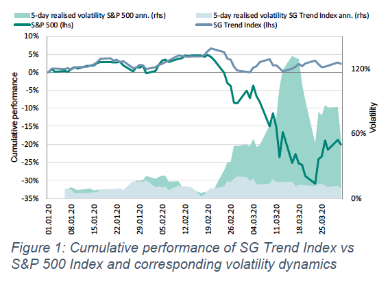
The second half of Q1 2020 turned out to be one of the most volatile periods ever for financial markets. The intensity and speed of the equity market sell-off has been unprecedented and market volatility has reached higher levels than during the peak of the financial crisis in 2008.
As one of few investment strategies, CTAs in general and trend-followers (TF) in particular fared well through the 2008 financial crisis, and also through the current Corona virus crisis period. The SG Trend Index returned +2.1% in the first quarter of 2020, while the S&P 500 was down 20% during the same period, as shown in Figure 1. Thus, CTA strategies and trend-followers have once again demonstrated their ability to provide diversification benefits to investors’ portfolios. At the same time, return dispersion between individual trend-following managers has rarely been higher than in these last couple of weeks.
The design of systematic trend-following programs involves many different building blocks, such as signal generation models, the structure of the investment universe, risk allocation targets between different asset classes, risk management models and portfolio construction methodology.
In this note, we analyze the impact on return dispersion of only one particular aspect of the design of a systematic trend-following model: the speed of the trend-following signal measured by the length of the look-back period used to capture trends, i.e. its velocity.
While it seems natural to assume that shorter-term models, which adapt quicker to a changing market environment, perform better during strong market reversals, we will quantify the return differences over this current and previous market crisis. In addition, we aim to quantify the long-term premium paid in return for the outperformance during crisis periods.
Introducing a generic trend-following model with four different signal speeds
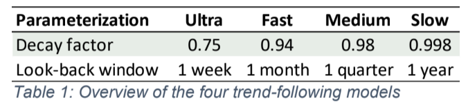
To perform the analysis we designed a generic trend-following model using a trend signal based on an exponentially weighted average of risk-adjusted past returns. We then applied a generic bottom-up portfolio construction method using a continuous, increasing and bounded risk-allocation signal function, and an implementation methodology aiming to minimize the number of transactions. This trend-following model is then applied to an investment universe of 62 of the most liquid futures contracts to obtain a portfolio return with an annualized volatility target of 12%. All simulated returns incorporate realistic trading costs of USD 40 per contract traded, but do not account for any roll costs, risk free return on cash, or any management and performance fees. Having specified the generic trend-following model, we will focus on the parameter of interest: the exponential decay factor, which reflects the speed or look-back window of the trend-following signal. The following four decay factors corresponding to different look-back windows will be considered.
The impact of signal speed and resulting equities allocation during the first quarter 2020 Figure 2 shows the cumulative returns for the four different model parameterizations between 20th February 2020 and 23rd March 2020, compared to the S&P 500 and the SG Trend Index. Table 2 provides the corresponding detailed breakdown of returns, risk and correlation metrics for that most volatile four-week period. Note how closely the generic Medium trend-following model tracks the SG Trend Index, as confirmed by a significantly high correlation of 0.88. Figure 2 and Table 2 illustrate the striking outperformance of the Ultra model over the slower models in March. The Fast model gained +6.8% over this four-week period, while the Medium model lost -5.4%. This corresponds to an enormous outperformance of 12% over this short period, which can simply be explained by the different decay factors.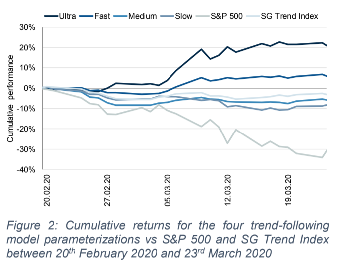 A great portion of the difference in returns between the various models is explained by the portfolios’ equity positioning, as highlighted by the asset-class return attribution in Table 2. Equities would have contributed +10.2% to the short-term Ultra trend-following model as a result of moving quickly from long to short. However, even the Fast model would have lost -4.2% over the same period from its equities holdings but still outperforming the Medium model by a striking 9.6%. Further, it is worth highlighting that all four models generated similar and positive returns in the remaining asset classes, an illustration of the importance of asset class diversification of any trend-following approach.
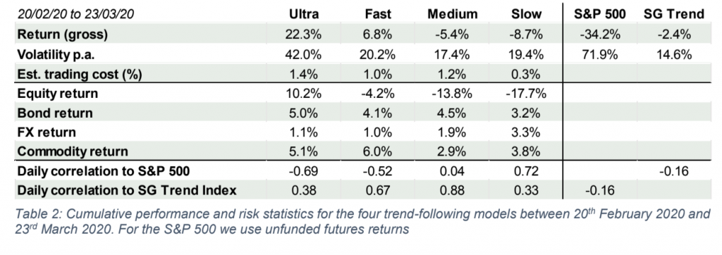
Figure 3 shows the dynamics of the equity exposures for the different models between 20th
February 2020 and 23rd March 2020. 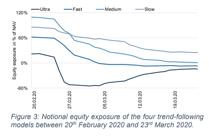
The Ultra model had already significantly reduced
long equity exposure by mid-February and took
considerable short positions of around -50%
notional exposure in the first week of March. All
other models reduced equity exposures
considerably in that first week of March, thus
limiting the losses in equities and allocating most
of the risk in other asset classes that generated
diversifying profits. These simulations indicate
that the positive return of the SG Trend Index in
Q1 was not a result of short positions in equity markets, but rather that of strong profits in diversifying positions, mainly long positions in bonds, short positions in energy markets and short positions in FX markets against the USD. Corona Crisis and the Financial Crisis of 2008: a comparison Looking back in time, the market environment that comes closest to the one we are currently witnessing is the financial crisis of 2008. How did the return dispersion – as a function of the speed of trend-following models – look like back then? Table 3 shows that, when analyzing our four generic models over the period from 1st January 2008 to 6th March 2009, dispersion was much less pronounced between the Ultra, the Fast and the Medium model. It was only the Slow model that underperformed considerably. Noteworthy is the correlation structure between the four models and the SG Trend Index, as illustrated in Figure 4.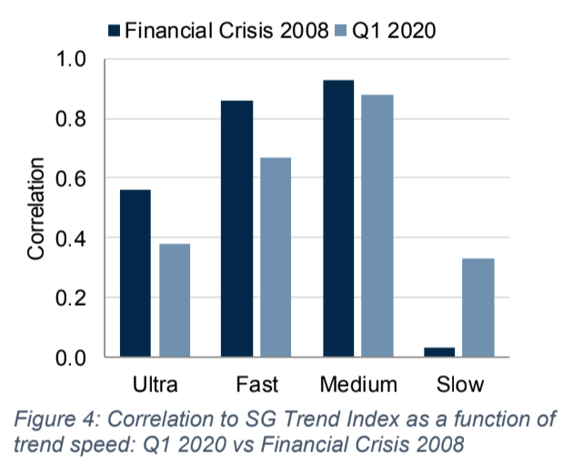
In 2008, our shorter-term models were more correlated to the SG Trend Index than they were more recently. In 2020 longer-term models have seen their correlation to the index increase vs their shorter-term counterparts. This supports a hypothesis often debated in our industry: There has been a tendency for the SG Trend Index constituents, which are the ten largest TF firms, to employ slower trend-following models in more recent times than in the previous decades.
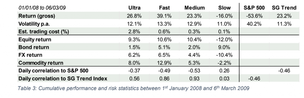
During the financial crisis in 2008, the allocation to equities had a much smaller impact on the dispersion of returns than it did in the first quarter of 2020. This illustrates the main difference between the two stock market crises: The Ultra model only was able to exploit the sheer speed with which the markets corrected in the first quarter of 2020, whereas during the 2008 crisis all but the Slow model made significant gains with their equity allocations. While it took the S&P 500 one full year to correct 30% from its previous high in October 2007 to the lows in October 2008, global equity markets corrected over 30% from the highs in mid-February 2020 in less than one month. Thanks of the speed and intensity of the risk repricing and associated volatility spikes
across all asset classes, March 2020 has provided exceptional market conditions for short-term TF approaches. As the current crisis is only five weeks young, it is, however, premature to draw some final conclusions from a comparison with the 2008 crisis.
Long-term results and smart diversification characteristics
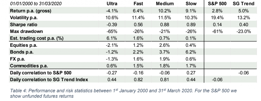
We extend the analysis and focus on the long- term results and smart diversification characteristics of the generic trend-following models with the four different look-back specifications over a long period starting in 2000. Table 4 provides a summary of key return, risk and correlation metrics.
While the Ultra model delivered strong returns during the two above mentioned crisis periods, it failed to deliver positive results over the long term (-4.1% p.a. between January 2000 and March 2020). Around half of the underperformance against the Fast model is explained by the additional transaction costs of around 4.5% p.a. versus the Fast model. The best long-term results are achieved by the Slow and the Medium model, with a (gross) Sharpe-ratio of close to 0.9 and corresponding transaction costs of less than 1% p.a. Over the 2008 and 2020 market crises the Fast model outperformed the Medium model by a combined 28%. However, this significant ‘crisis alpha’ comes at a long-term premium that amounts to +3.8% p.a. over the last 20 years, or
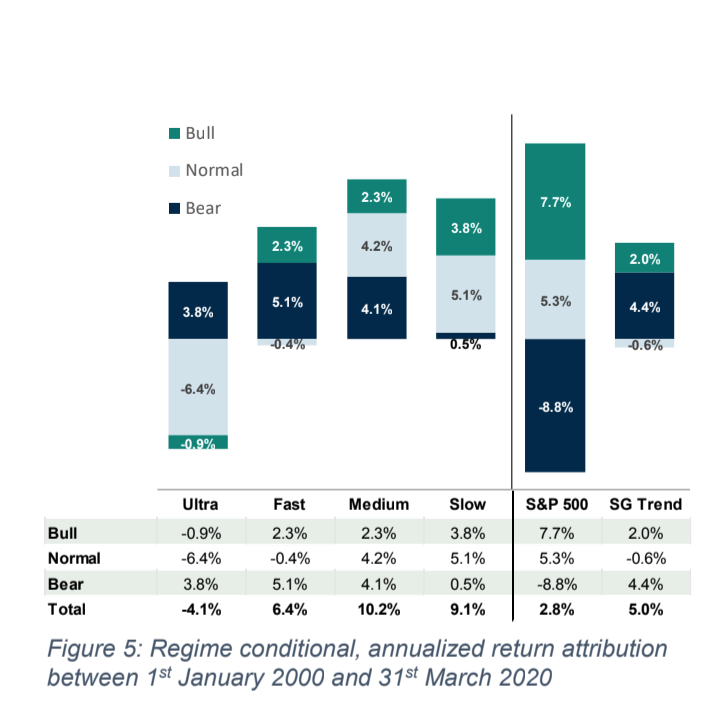
an estimated Sharpe-ratio discount of 0.32. In order to gain a deeper understanding of the behavior of the different model specifications in different market environments, we perform a regime conditional return analysis and follow the definition and approach as in Trend-Following CTAs vs Alternative Risk-Premia1. In short, three different market regimes are defined based on non-overlapping quarterly returns of an equity market benchmark (we use the S&P 500 futures returns): a Bear market regime, a Normal market regime and a Bull market regime2. Figure 5 shows such regime conditional return attribution.
It highlights an important and well-known feature of trend-following programs: Independent of their speed, trend-followers have offered strong downside protection over the last 20 years, demonstrated by the positive returns generated in the Bear market regimes. Historically, this crisis protection has been higher for the Ultra and the Fast model, but this comes at a cost: While on
average longer-term trend-following strategies manage to deliver positive returns in all three regimes, the Ultra model, and less so the Fast model, suffered painful losses in a “non-crisis” or “Normal” market regime (in 68% of the quarterly return sample). Faster trend-following programs hence pay a premium for downside protection that is a combination of higher trading costs (due to higher turnover) and multiple false signals if short- lived corrections do not develop into a significant crisis. Slower trend-following models still provide positive, but smaller crisis protection and deliver significantly higher returns in Normal market regimes.
Conclusion
While faster trend-following strategies are particularly well suited to adapt and profit from sudden market distress, medium- to long-term approaches offer a more consistent risk-return profile across different market regimes by better capturing long-term returns and still offering great diversification benefits. According to our historical simulation, the generic Medium model with a lookback window corresponding to one quarter delivered the highest long-term Sharpe-ratio, and the best balance between crisis protection in Bear markets and positive participation in Normal and Bull markets. It generated significantly positive results in all three different market regimes over the long-term, hence offering the most efficient smart diversification benefits.
Return dispersion between trend-following managers is the result of large variations in the design specifications of a systematic investment process. In this note we focus on one aspect of the model design only – the speed or look-back period of trend-following signals.
We show that different look-back specifications can lead to a return dispersion of up to 30% over just a few weeks in an extreme scenario as witnessed during the first quarter of this year. Even a relatively moderate increase of the look-back period from one month to one quarter can explain an underperformance of more than 12% within one month. We further demonstrate that the beneficial drawdown protection of faster models comes at a price, or a long-term premium.
References
1 For details on specifications of regimes relative to any
benchmark we refer to Artur Sepp and Louis Dezeraud (2019), “Trend-Following CTAs vs Alternative Risk- Premia: Crisis beta vs risk-premia alpha”, The Hegde Fund Journal, https://thehedgefundjournal.com/trend- following-ctas-vs-alternative-risk-premia/2
In particular, we term market regimes 1. as Bear regimes when returns on the
benchmark are below the 16%-quantile; 2. as Bull regimes when returns are above the
84%-quantile; 3. as Normal regimes when returns are in-between
the 16%- and 84%-quantiles. The justification for using a 16%-84% range is that these
Related Posts

Navigating Economic Crossroads: A Closer Look at the Unconventional Path
In the famous Robert Frost poem “The Road Not Taken,” two paths diverged, and he took the one less traveled. We can look at charts of the US economy and compare them to previous periods to see that so far, we are taking the less traveled path as well. It makes all the difference. Despite […]

Cargo Collapse Chronicles: Navigating the Economic Storm through Freight Industry Signals
Economists often look for the proverbial “canaries in the coal mine” to predict where we head next. Specific areas of the economy tend to presage slowing growth earlier than others. The shipping of materials from one place to another is one such area. A supply chain is either gearing up for future sales or reducing […]

Ag Market Update: Wheat Prices Drop, China Becomes Top Wheat Importer, and Soybean Complex Dynamics
Commentary provided by Chad Burlet of Third Street AG Investments For corn and soybeans, it was a quiet harvest month as far as prices were concerned. Futures contracts for both crops had only 5-7% trading ranges and settled within 1% of where they were a month ago. The U.S. harvest is progressing well, with both crops ahead […]